 (Click
to enlarge)
(Click
to enlarge)
Click on any of the following images for a full view.
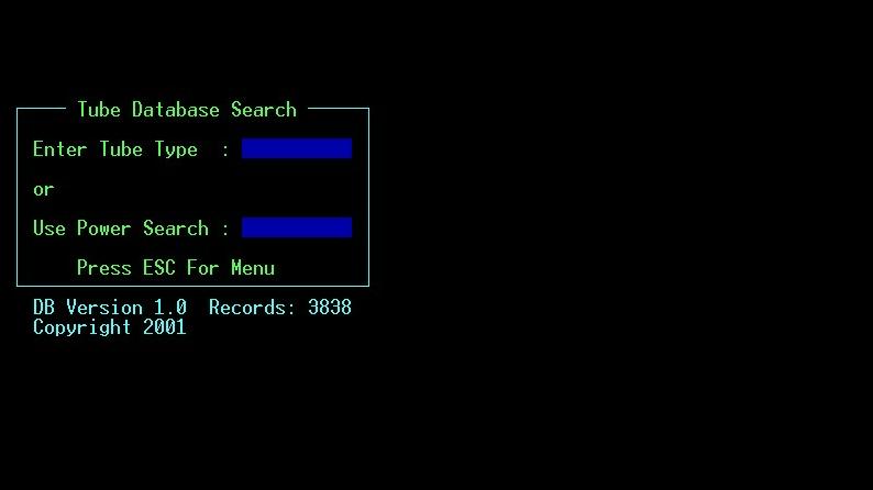
When the software is launched, this is the first screen we see (the search screen):
Simply type the number of the tube to be tested into the upper field (fields are areas which you can type in and they are usually blue) and then press ENTER. If desired a partial number may be entered. The lower field, Power Search, is used to search the database more thoroughly and also lets us use the program as a cross reference (more on this later).
Suppose we type in KT66 and press ENTER. Here is what we are presented with:
Whoa! There is a lot of information here, but don't let that scare you. In fact, if all we wanted to do is test this tube, we wouldn't be concerned with anything on this screen except to confirm that we have pulled up the right tube and the number of tests involved. We would simply press the "T" key (for Test) and we are testing. Now that's fast! At this point the tester is operating just like we had inserted the KT66 test card. We complete the testing procedure just like we normally would on any Cardmatic:
1) - Check for shorts by observing the tester's short lamps, and
read the meter to check for any heater to cathode leakage
2) - Perform the quality test (press button 2 and read the meter)
3) - Perform the gas test (press button 3 and read the meter)
That's it! It really is that easy to use. If we wish, we can convert the meter reading obtained during the quality test directly to uMhos by consulting the color coded meter conversion chart on the right side of the screen. If the tube has more than one test, we press the space bar to take us to the next test. Pressing ESC takes us back to the search screen and we are ready to test the next tube. If all you want to do is test tubes, you are done. You have now been granted an Associates Degree in Tube Testing and may leave. But, if you want to do more, read on.
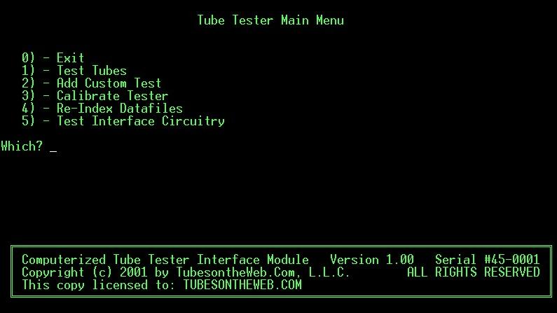
The rest of the information on the screen is there only if we need it (or are curious). For example, after studying the test parameters we may decide that for our application a more accurate test could be performed if we changed the conditions under which the tube is being tested. To achieve this, we can easily add a test to the database that uses our own parameters. Let us do that by pressing ESC to return to the search screen, then pressing ESC again to get to the main menu (pressing ESC from anywhere always takes us back). Here is what the main menu looks like:
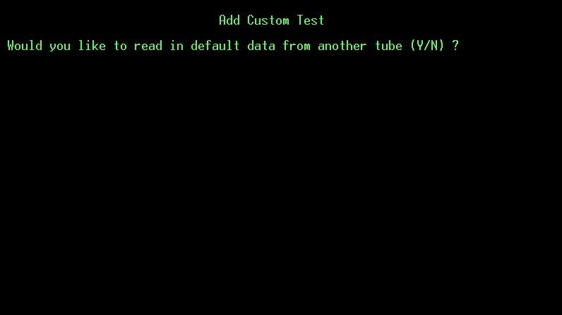
There are several options. For now, we will select item 2, "Add Custom Test", so we can input our modified KT66 custom test. Here is what we see:
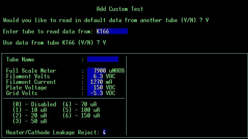
Since we will still be testing a KT66, we should answer this question "Yes" and tell it to read in the data from the KT66 already in the database. That way things like the type of test, pin out, and filament voltage are already properly set for us. If this question is answered "No", then we could change things like the type of test (Transconductance or Plate Current) and bias mode (grid or self). For now we will answer yes, then tell it to read in the test data from the KT66 already in the database:
In this case we are looking at a Transconductance test using grid bias. What we will change is the plate voltage. We are going to set it at 180V. Unfortunately we can't go much higher because we start to run into the limits on the amount of current we can draw from the regulated B+ power supply. We will also need to increase (make more negative) our negative grid bias to keep the tube's operating point within the proper range for the gm measurement bridge circuit.
We start by giving it a name. This one we will call KT66Spl (for KT66 Special), and we will change the parameters just mentioned. When we have filled in all the fields and reached the bottom of the screen, the program asks us to confirm our changes. After pressing the "Y" key, it stores our test in the database along with all the other tests. The original KT66 test is still there too, untouched. Now lets go back to the search screen, pull up our newly entered custom test, and look at it in more detail:
First we will discuss at the upper section on the screen. It contains three fields of information that we can edit if we wish: the type number, an optional alternate type number, and a place for remarks. The type number is simply the number that the tube is known as. The alternate number is used when a tube is also known by a second number. For example, the 6BQ5 is also known as an EL84. This alternate number field is included in the search when using the Power Search that we mentioned earlier, which is how the program functions as a handy cross reference. Next, the remarks field is used for anything we might need to know. For example, a test might be one that measures a tube's ability to achieve complete cut off, and any reading under 50 on the meter indicates a good tube. In that case the remarks field will say "OK UNDER 50", so it is important to pay attention to this field. In fact, if there is something in this field it will turn red in order to draw our attention to it. We can add to it anything we like, but please do not change anything that is already in this field. The upper section also shows the total number of tests involved for this tube and which test we are currently on.
The right side of the screen holds the meter conversion chart. In this case it is a transconductance test so we can convert the meter reading directly to micromhos by consulting this chart. If this were a current or voltage test, the chart would convert directly to mA or volts for us. The chart is color coded: good tubes will register in green numbers, marginal in yellow, and failing in red. It is a sliding chart that adjusts automatically to match the test. At the bottom of the chart there is a notice that the letter "O" key (stands for Odd/Even) can be pressed at any time to toggle the chart between odd and even numbers.
The left side of the screen shows what tester line is connected to what tube pin. This is worded as "tester line" intentionally because these lines are not always used for what they seem. The tester's circuits are so versatile that it is sometimes handy to use a line for something other than what it is labeled as. Do not design your circuits using the pin out shown on this screen!
The central area of the screen shows the test parameters. Some of these fields change depending of the type of test being performed. In this case most of the parameter fields can be edited, or changed, because this is our custom KT66 Special test that we added earlier. These fields cannot be changed in the 3800+ tests that come with the tester. Of particular interest is the "Adjusted Filament Voltage" field. This is the voltage actually being chosen from the filament transformer taps, and is based on the amount of filament current being drawn. It makes up for the voltage drop in the wiring so that the tube receives the proper filament voltage at the pins. Low filament voltage, especially on low voltage high current tubes, has always been this tester's biggest weakness. This problem has been completely eradicated since the computer picks the right voltage automatically!
At the bottom of the screen are the commands we can use. They are all one key commands, so all we need to press is the key indicated in parentheses. Let's take a look at each, in order. The first, (C)urves, will be saved for the end of this discussion. The next command, (D)elete, is pretty much self explanatory, and appears only on custom tests. None of the tests that are originally supplied in the tester's database can be deleted.
Next, (E)dit, is used to change any fields on the screen that are allowed to be changed. This command is very simple. When the "E" key is pressed, the cursor moves up to the top field. Make any changes needed using normal editing keys (delete, insert, etc.). Use ENTER or the down arrow key to skip any fields that do not need changes. Use the up arrow key to get back to a previous field. After making changes, either press ENTER repeatedly to get to the bottom of the screen, or press Page Down to skip the remaining fields. If one or the other isn't done, or ESC is pressed after making changes, then the changes will not be saved.
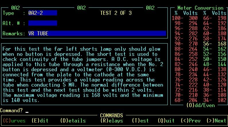
The (I)nstructions command is needed only if you have not read this document. Pressing the "I" key in this case will give us only generic instructions that have already been covered. On the other hand, if there are instructions that are specific for the tube being tested (such as most voltage regulator tubes), then the instructions will automatically pop up in the central area of the screen when you first call up that tube. For example, here is the 0A2 test screen:
As you can see, the parameters that are normally presented in the central part of the screen have been replaced with instructions specific for this test. Also a new command, (D)etails, has appeared that can be used to switch from the instructions to the familiar parameter display that is normally in the central screen area.
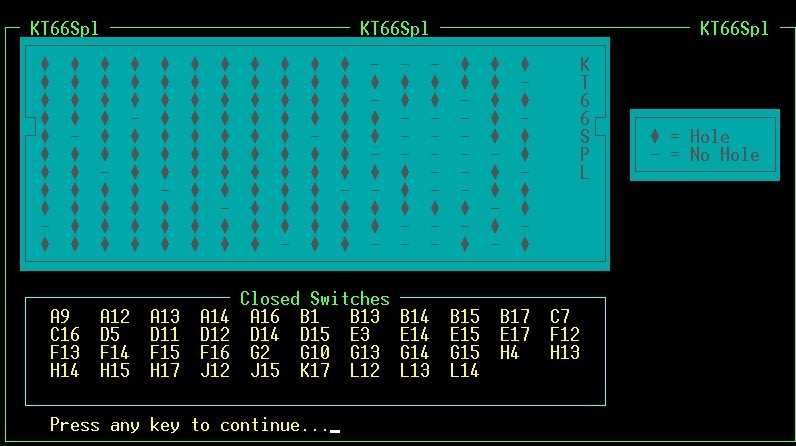
The next command, (R)elays, is a screen that shows which switches (relays) are closed for this test, and a graphical representation of the card, if we cared. This screen is used only for diagnostic functions:
The all important (T)est command is next. Simply insert the tube into the tester and press the "T" key to start the test. The actual test procedure was covered earlier, but one test that was not mentioned is the sensitive grid shorts test. There is a button under a hinged cover on the right side of the tester labeled "Sensitive Grid Shorts". If critical audio tubes are being tested, it is a good idea to use this test. Simply press the button and observe that no short lamps start glowing.
The rest of the commands are simply (Q)uit, which exits the program completely, and representations of the left and right arrow keys, (<) and (>), which lets us quickly move backward and forward through the tube database in numerical order. For example, to bring up our KT66Spl test, we could just type KT66. Then the KT66 test screen (the original one) pops up, and pressing the right arrow key makes the program go to the next test, which in numerical order is the KT66Spl test we are looking for.
Are you still wanting more? Good, because now we are going to talk about curves!
First, we will be going through the process of setting up the curve test parameters for our newly added KT66 Special, but don't get confused here. The set up procedure we are getting ready to discuss can be tedious, but once completed the process of creating the curve charts themselves is quick and easy (much easier than the initial setup procedure). Here is a quick overview of the curve trace process, once the parameters have been set up:
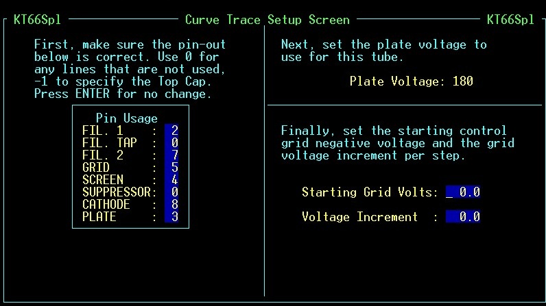
To look at these steps in detail, we will start with our KT66 Special that we already have pulled up on the screen. When we press the "C" key, one of two things will happen. Normally, a tube will already have had its curve test parameters entered, in which case the program will take us directly to the curve trace test screen. However, these parameters have not yet been set up for our KT66Spl, so when we press the "C" key we are taken to the curve setup screen:
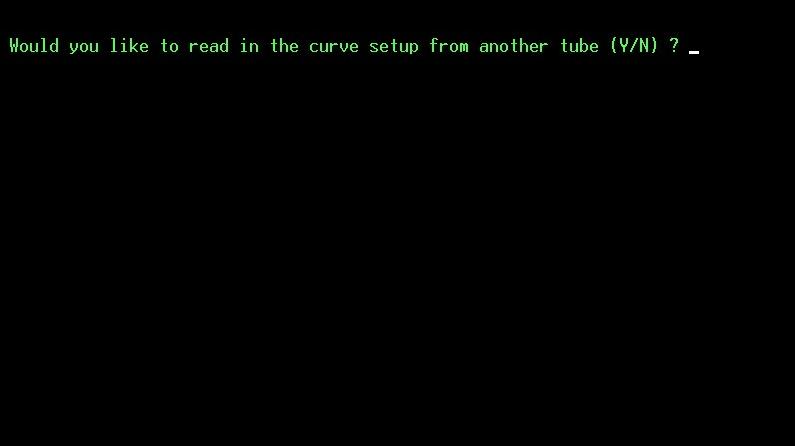
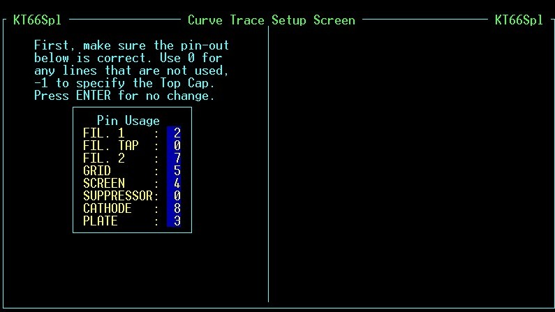
Hopefully, to save time, there will be other tubes with similar characteristics that already have their curve parameters entered. If so, we can read the default data in from one of them. Setting up a good curve is usually a process of trial and error. Fortunately, once a curve is set up for a particular tube, it is stored in the database. Many common audio tubes already have the curve test parameters set up. But for now, let's answer "No" to this question and setup a curve from scratch. This takes us to the first part of the setup process, the tube's pin out:
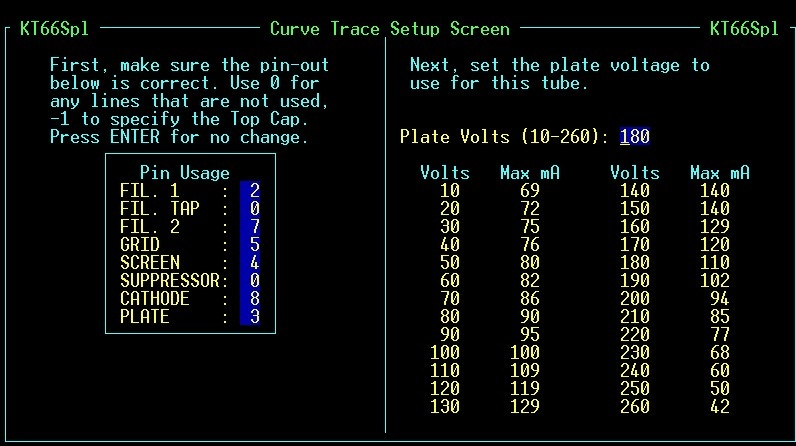
Remember the program can only guess at the pinout. Even though most of the time it will be right, it is important to consult a tube manual or schematic at this point to verify that the pin out is correct. After making sure it is correct and/or making any necessary changes, we can continue to the next part of the curve setup process, selecting the plate voltage:
Our choices range from 10 volts to 260 volts. A chart is presented that shows the current limit of the B+ supply for any given voltage. As you can see the maximum available current peaks at 150 volts, which is why 150 is the most common plate voltage used for testing. You can exceed these limits by about 20% before the B+ regulation starts to suffer appreciably. We decide to try a plate voltage of 180 volts, so that is what we'll enter. Now, for the last part of the set up process, we need to enter the starting grid bias voltage and the amount to increment this voltage for each test:
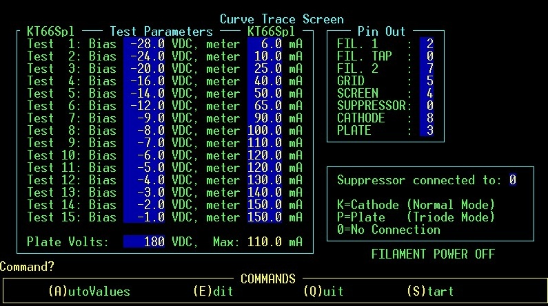
This is the toughest part to decide on. Use your best judgment based on your experience with the characteristics of the tube type being set up and the plate voltage you selected. If you don't have any experience, just guess and don't worry about it, because you will almost certainly have to tweak the values later anyway. In this case we are going to enter a starting voltage of -16 volts, and a voltage increment of 1 volt per test (more on why we picked these values later). After entering these initial values we are now finished setting up the curve parameters for this tube. The program automatically takes us to the curve trace test screen:
Actually, the screen you see here has already been edited with the final values decided upon by using a trial and error method. That is why we don't see the bias for the first test starting at -16 volts and proceeding with 1 volt increments like we specified a moment ago on the set up screen. Since tubes are not very linear near cutoff, all properly set up curves have relatively large grid voltage increments for the first several steps. As you can see, most of the grid bias voltage increments really are 1 volt apart once we get several steps into the tests. When setting up new curves, pick a starting bias voltage based upon where you want the last test's bias voltage to be, not on where the first test will actually begin. In this case it was decided to have the last test's bias at -1 volt. Since there are 15 tests and the voltage increment is 1 volt, we started at -16 volts. This resulted in the last test being at -1 volts (-16 + 15 = -1). Note that not all curves need to be set up using all 15 tests, but the more we use the more accurate the results. You must use at least 8 tests.
Notice there is an option for where to connect the suppressor grid. If we are testing a pentode, we can connect it to either the cathode (normal connection) or the plate (triode connection). If we wished to change this setting we would use the (E)dit command to do so. When the chart is printed it will indicate whether the curve was done in normal mode or triode mode. The screen grid, if applicable, is always connected to the plate during these tests.
Lets quickly look at the commands available at the bottom of the screen. First is (A)utoValues, which simply allows us to choose a different starting bias and/or increment voltage and then fills in the fields with these new values. Use it to save typing if the bias values are so far off that they all need to be changed. Next is (E)dit, which will allow any setting on the screen to be changed. (Q)uit takes us out of the curve trace test screen and back to the normal test screen (pressing ESC does the same thing). Finally, (S)tart actually starts the series of tests. Lets press the "S" key see what happens:
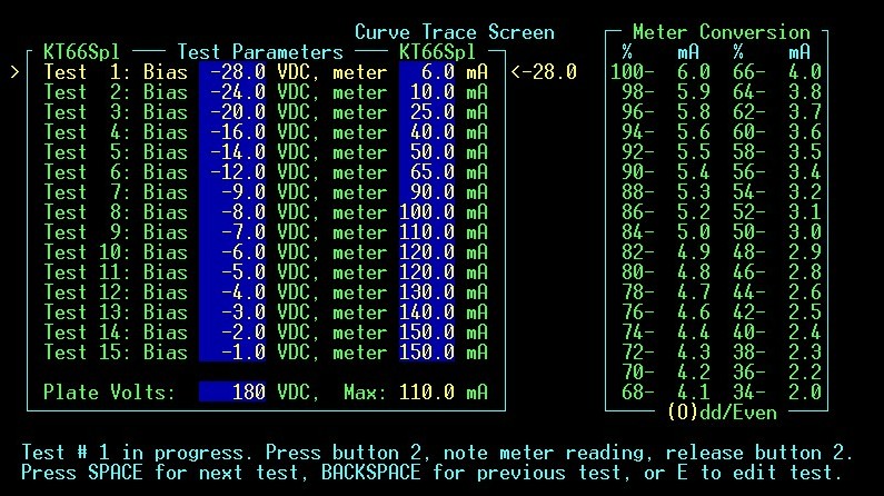
Notice that the meter conversion chart is back. It is not really necessary, but we can use it to tell how much B+ current we are drawing for the particular test we are on. The numbers in the meter conversion section will turn yellow once the B+ power supply's rated current has been reached. They will turn red once 120% of the rated current has been reached. If we reach the red numbers, then the meter readings cannot be trusted and we will need to edit the curve parameters to reduce the amount of B+ current being drawn.
Now that we finally have the curve tests underway we simply press button 2, note the meter reading, release button 2, then press the space bar. The program will ask us to enter the meter reading before moving on to the next test. If we need to go back to a previous test for some reason, we can press the BACKSPACE key. It is easy to tell which test we are on because it is highlighted in yellow and has the applied grid bias voltage printed to the right. This procedure is repeated until all the tests have been performed.
If at any time during this procedure we need to change the parameters of the test we are currently on (which we will since this is the first time this set of curve tests have been used and the meter sensitivity settings will almost certainly be wrong), we can press the "E" key. This will allow quick editing of the bias voltage and/or the meter sensitivity of the current test only. When setting the meter sensitivity, it is recommended that a value be selected that results in a meter reading of between 50 and 60 for a typical tube. This gives an accurate current measurement while providing enough meter scale leeway to allow for unusually strong tubes.
Once all the tests have been completed, the program will ask to save the data. When told "Yes", the program will prompt us with the tube's serial number. This is simply a sequential number used to identify individual tubes. It is also the name given to the file that the curve data is stored in. The computer will automatically increment and remember this number, so we can just press ENTER to accept the number the computer assigns. We also need to mark the tube itself with this number. We are also given a chance to enter some remarks which are put at the top of the chart printout. It is usually used to describe the tube (brand, new/used, construction, etc).
The last question we are asked is where to save this data file. Here is what the screen looks like once we reach this point:
If the program is being run on the same computer that will be used to print the curves, meaning that it is a Windows based computer that has Microsoft Excel loaded, then it is recommended to save the data files in C:\MYDOCU~1\ (the way DOS sees the C:\My Documents\ folder). This is because the Excel macros look for the files there. If the files need to be transferred to a different computer for display and/or printing, then save them to a floppy disk (A:\). The program remembers where the last file was stored, so after telling it the proper location once we can just press ENTER to accept the default in the future.
During this whole procedure of editing and testing the filament power was always on. This allows for quickly moving through the tests since no warm up time is needed between tests. The filament power is not removed until either the tests are successfully completed and the data stored or the curve trace screen is exited. There is a prompt displayed on the lower right portion of the screen that shows at any given time whether or not the filament is powered.
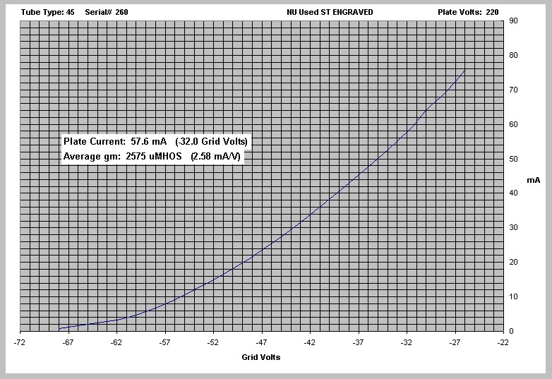
We are now through curve tracing this tube, and can move on to the next tube. We can do as many as we like in one setting even if we are storing them on a floppy disk (the files are very small). Once you get the hang of it you can create curves for a lot of tubes in a short time. The macro that prints these curves will print all of them with just one keystroke. Here is the curve for a typical type 45 tube::
These curves are great for a couple of reasons. We can look at the line itself to see if the tube under test is nonlinear in any way (this one is excellent). We can use the information printed in the upper left portion of the chart to create some very well matched pairs and quads of tubes. The software produces this information by using the curve itself, resulting in an exquisitely sensitive test. For the plate current, a point two thirds of the way up the curve is chosen, and the current measured at that point is used (in this case the two thirds point is at -14 grid volts). The average gm is calculated by measuring the average gradient of the curve starting at 2 grid volt "increments" down from the two thirds point and ending 2 increments up from the two thirds point (an increment being the voltage increment we used during the curve tests). It is interesting to see how individual tubes show their differences here, when otherwise they test as matched. Click here for more information on what defects these charts can show you.
Isn't this great stuff? There is even more information (including tester calibration) covered in the White Paper. But since you made it this far, you are now awarded a full Honorary Master's Degree in Computerized Tube Testing and Curve Tracing!
Thank you for taking the tour!